Preprocessing of Illumina methylation arrays in CpGene follows a structured and quality-controlled workflow based on the minfi framework, ensuring high data integrity and reproducibility before any downstream analysis. Raw IDAT files are imported alongside the sample sheet, which provides metadata and identifiers linking each array to its biological condition. Quality control begins with the computation of probe-level detection p -values, which quantify the confidence that measured intensities differ from background noise. The mean detection p -value across all probes is calculated for each sample, serving as an indicator of overall assay quality. Samples exceeding the established threshold are excluded, thereby eliminating low-confidence data that could bias subsequent analyses. Assay performance is further assessed using control probes designed to monitor bisulfite conversion efficiency across both color channels, as well as by examining global quality metrics that summarize intensity distributions per sample. Once poor-quality samples are removed, normalization is applied through a control-probe–informed approach that corrects for between-array technical variability while preserving biological differences. This method begins with a background correction step that models non-specific fluorescence using a combined normal–exponential framework. Here, background noise is assumed to follow a normal distribution, while the true methylation signal is modeled as exponentially distributed. Out-of-bound probe data—fluorescence measured from the inactive color channel of Type I probes—provide an empirical estimate of background levels for each sample. By subtracting this modeled background, the resulting intensities more accurately represent the true methylation signal. Following background correction, the workflow applies principal component analysis (PCA) to the control probe intensities to capture dominant sources of unwanted technical variation, such as batch or hybridization effects. The first principal components are then used to adjust probe intensities, effectively removing systematic technical noise while maintaining biological signal integrity. This combined background correction and PCA-based normalization strategy has demonstrated high performance in studies involving strong biological contrasts, such as comparisons between cancer and normal tissues or heterogeneous cell types. It ensures that the resulting β-values are technically consistent and biologically meaningful. After normalization, several filtering steps are applied to retain only high-confidence CpG probes. Probes that fail the detection p-value threshold in any remaining sample are removed to eliminate unreliable measurements. Loci overlapping known single-nucleotide polymorphisms are excluded to prevent genotype-driven artifacts. Additionally, published catalogs of cross-reactive probes—those that hybridize to multiple genomic locations—are used to further refine the dataset. The remaining β-values are then examined to confirm their expected bimodal distribution, reflecting hypomethylated and hypermethylated states across samples. CpG sites that fall consistently within the intermediate hemi-methylated range (β-values between 0.3 and 0.6) are excluded, as they typically represent ambiguous methylation states and contribute limited discriminatory power to downstream analyses.

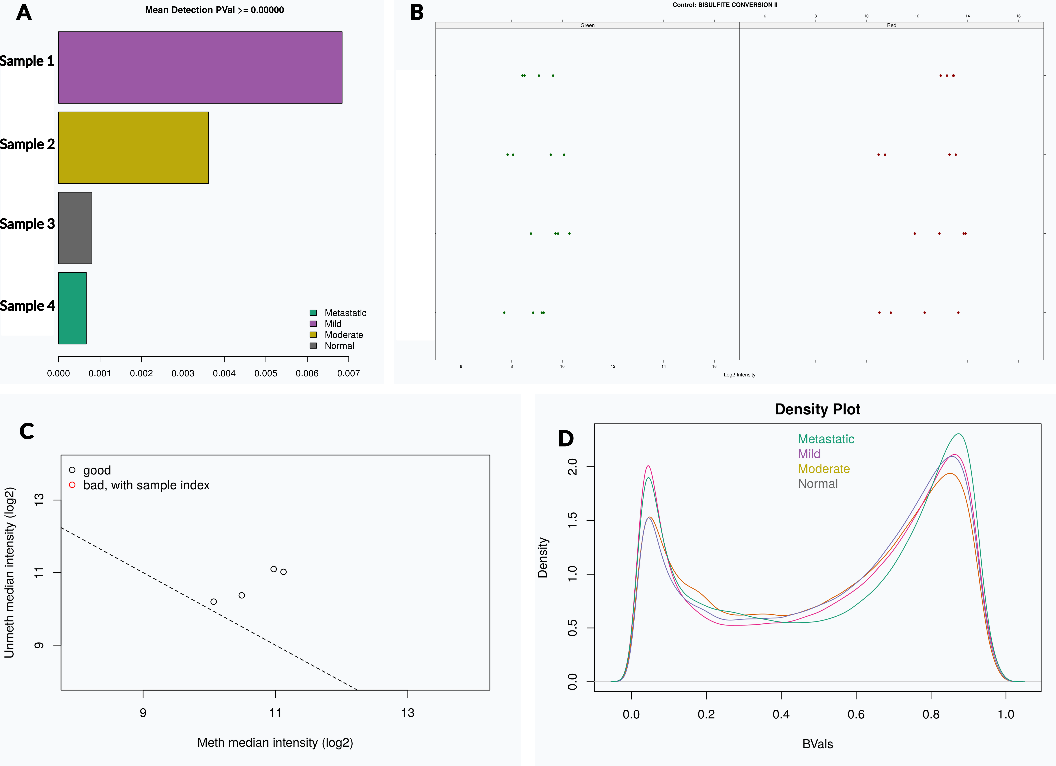
Figure 1. (A) Mean detection p -values per sample, with color-coded categories indicating clinical groups. Samples exceeding the detection threshold were excluded from further analysis. (B) Control probe performance for bisulfite conversion type II, shown across both red and green channels, confirming consistent conversion efficiency. (C) Median methylated versus unmethylated signal intensities used for identifying low-quality samples based on overall signal distribution. (D) Density plot of β-values across all samples and groups following normalization and filtering, illustrating the expected bimodal distribution corresponding to hypo- and hypermethylated CpG sites.

The growing complexity of high-throughput biological data, especially from DNA methylation arrays, has created the need for more advanced computational methods in biomarker discovery. Modern array platforms measure hundreds of thousands of CpG sites, creating a large imbalance between the number of features and the number of samples, often referred to as the curse of dimensionality. This imbalance can make it difficult for traditional statistical techniques to identify meaningful patterns. To address these challenges, CpGene uses a set of artificial intelligence–based feature selection methods, including the Garson Olden MLP, Ridge Classifier with L2 regularization, Recursive Feature Elimination (RFE) with an SVM classifier, SHAP with XGBoost, Random Forest Variable Importance, and Logistic Regression with Lasso.

Feature selection using the Garson–Olden Multilayer Perceptron (MLP) method in CpGene quantifies the relative contribution of each CpG site by propagating connection weights through the trained network. Once the MLP model is fitted, each neuron’s influence on the output is expressed through the absolute magnitudes of its connection weights. For a network with one hidden layer, the importance of an input feature can be computed as :

where $w_{ih}$ denotes the weight connecting input neuron to hidden neuron , represents the weight connecting hidden neuron to the output layer, is the number of hidden neurons, and the total number of inputs. This expression captures the cumulative strength of all weighted paths linking each input to the output, thereby reflecting its relative influence on the prediction. In deeper networks, this principle is extended by recursively multiplying the absolute values of weight matrices across layers, yielding a generalizable metric of importance that can handle non-linear feature interactions (Garson, 1991; Olden et al., 2004). To ensure stable and reproducible feature rankings, the model is trained repeatedly using different random seeds, and the resulting importance vectors are averaged. This reduces the effect of stochastic variations inherent to neural network initialization and training. The final ranked list of CpG sites reflects features that exert the most consistent influence across trained models, providing interpretable and biologically relevant markers for subsequent mapping and enrichment analyses.

Feature ranking using Recursive Feature Elimination with a Support Vector Machine (RFE-SVM) ( Azman et al., 2023 ) is based on iteratively training a linear classifier to quantify the relative contribution of each CpG site to the discrimination between biological conditions. In this framework, a linear SVM learns a decision boundary defined by a hyperplane that maximizes the margin between classes. Each CpG site is assigned a coefficient , representing its contribution to the separating hyperplane. The absolute magnitude serves as an indicator of importance, as features with larger coefficients exert greater influence on the classification. At each iteration , the feature importance scores are computed as

where $w_j^{(t)}$ corresponds to the weight of feature j at iteration t. The features with the smallest $s_j^{(t)}$ values are then removed, and the classifier is retrained on the remaining subset. Repeating this process yields a complete ranking of features from most to least informative, allowing the identification of CpG sites that contribute most consistently to class separation. This methodology offers both interpretability and robustness, as the linear SVM provides a direct link between model coefficients and biological variables. The elimination process progressively refines the feature space by removing redundant or weakly contributing CpG sites, ultimately producing a ranking that reflects their discriminative strength. Mathematically, the decision function of the SVM is expressed as

where $\mathbf{w} = [w_1, w_2, \ldots, w_p]$ denotes the weight vector and $b$ the bias term. The recursive nature of RFE ensures that only features maintaining high $\lvert w_j \rvert$ values across successive iterations are retained near the top of the ranking, capturing the most biologically relevant methylation markers for further analysis and interpretation.

Feature ranking with Random Forest variable importance (Huang and Chen, 2021) relies on how much each CpG site contributes to improving class separation across an ensemble of decision trees. During training, each tree partitions the samples by selecting splits that reduce node impurity (e.g., Gini impurity). The importance of feature jin a given tree tis computed as the sum of impurity decreases produced by all splits on that feature, each weighted by the fraction of samples reaching the split:

where $S_j^{(t)}$ is the set of splits on feature j in tree t, p(s), is the proportion of training samples at the split, i and is the node impurity (for Gini, , $i(n) = 1 - \sum_k p_k(n)^2,\ \text{with } p_k(n)$ the class proportion at node ). The Random Forest importance is then obtained by averaging over trees and normalizing so that $\sum_j \text{Imp}_j = 1$. This yields a direct, model-based measure of how strongly each CpG site contributes to reducing classification uncertainty across the ensemble. In practice, the procedure produces a complete ordering of CpG sites by descending importance. Aggregation over many trees improves stability in high-dimensional settings and reduces sensitivity to individual partitions. It should be noted that impurity-based importance can distribute credit among correlated features and may favor variables with many possible split points; these effects are typical of tree-based models and can be contextualized alongside domain knowledge or complementary ranking methods if needed. The resulting ranked list highlights CpG sites that consistently drive impurity reductions across the forest, providing an interpretable basis for downstream gene mapping and pathway analysis.

Feature ranking with Ridge (L2-regularized) classification ( Khan et al., 2019 ) uses the magnitude of the model coefficients as an index of each CpG site’s contribution to class discrimination, while the L2 penalty stabilizes estimates in the high-dimensional setting. For a binary problem, Ridge learns a weight vector w by minimizing a penalized loss of the form

where $\mathcal{L}$ is a convex classification loss and $a > 0$ controls shrinkage of coefficients toward zero. In the linear setting, larger absolute coefficients indicate features that exert stronger influence on the decision function $f(\mathbf{x}) = \mathbf{w}^{\top} \mathbf{x} + b$. For multiclass classification, the model yields one coefficient vector per class in a one-vs-rest formulation; feature importance can then be aggregated across classes by combining the class-specific absolute coefficients. To obtain a stable ranking that is less sensitive to sample fluctuations, the procedure repeats model fitting over multiple random subsamples of the rows and averages the resulting coefficient magnitudes. Denoted by $\mathbf{w}^{(r)}$ the coefficient vector estimated on repeat $r = 1, \ldots, R$ , the stability-averaged importance for feature in the binary case is

Sorting features $s_j$ by from largest to smallest yields a complete ranking of CpG sites. The L2 penalty reduces variance and distributes weight among correlated predictors, while the repetition-and-averaging step enhances robustness, providing a practical and interpretable pathway to prioritize methylation markers for downstream analysis.

Feature ranking with SHAP values for gradient-boosted trees quantifies each CpG site’s local contribution to model predictions. For a fitted XGBoost classifier (Zhang et al., 2023) with prediction function f(x), SHAP assigns to every feature j and sample i an additive attribution $\varphi_{ij}$ such that

where $\varphi_{i0} = \mathbb{E}[f(\mathbf{X})]$ is the model’s expected output. Each $\varphi_{ij}$ is the Shapley value of feature computed over all coalitions of features, capturing its marginal contribution to the prediction while preserving local accuracy and consistency. For tree ensembles, TreeExplainer computes $\varphi_{ij}$ efficiently by aggregating path-dependent contributions across trees, avoiding brute-force enumeration of coalitions. In multiclass settings, attributions are defined per class; they can be arranged as $\Phi_i \in \mathbb{R}^{K \times p}$ and then combined across classes (e.g., by averaging absolute values). To obtain a global importance score for ranking CpG sites, per-sample attributions are summarized by the mean absolute SHAP value,

or, in the multiclass case, $S_j = \mathbb{E}_i\!\left[\frac{1}{K}\sum_{k=1}^{K} \lvert \varphi_{ij}^{(k)} \rvert\right]$. Sorting features by $S_j$ yields a complete ordering from most to least influential on model output. When two features have similar $S_j$, a secondary, model-internal criterion such as XGBoost’s split gain (the average loss reduction attributable to splits on a feature) can be used to break ties. The result is an interpretable, model-consistent ranking that reflects both local and global impact of CpG sites on predictions, suitable for downstream gene mapping and enrichment analysis.

Feature ranking with Lasso‐regularized logistic regression treats each CpG site’s coefficient as a direct measure of contribution to class discrimination, while the penalty promotes sparsity ( Friedman et al., 2010 ). For a binary outcome, the model fits a linear decision function $f(\mathbf{x}) = \mathbf{w}^{\top}\mathbf{x} + b$ and estimates (w,b) by minimizing the penalized negative log-likelihood

where $\sigma(z) = \frac{1}{1 + e^{-z}}$ and $λ>0$ controls sparsity. The $\ell_{1}$ term drives many coefficients exactly to zero, yielding an embedded selection of CpG sites that most strongly affect the log-odds of class membership. In the multiclass case with K classes, a one-vs-rest formulation produces class-specific weight vectors $w_{1}, \ldots, w_{K}$ with the same penalized likelihood principle applied per class.

Feature importance is then derived from the fitted coefficients. For binary classification, the absolute magnitude $\lvert w_j \rvert$ serves as the importance of feature j; larger values indicate stronger influence on the decision function. For multiclass outcomes, a common aggregation is the coefficient vector norm across classes, e.g. $s_j = \bigl\lVert [\,w_{1j}, \ldots, w_{Kj}\,]^{\top} \bigr\rVert_{2}$, which summarizes how much feature contributes across all one-vs-rest problems. Sorting features by these scores yields a complete ranking from most to least informative. Because $\ell_{1}$ regularization can distribute weight unevenly among correlated CpGs, simple secondary criteria based on feature–response association (e.g., correlation with class indicators) can be applied to break ties between features with similar primary scores, leading to a stable and interpretable ordering for downstream annotation and enrichment analysis.

In all implemented feature selection methods, users are provided with the option to specify the number of top-ranked CpG sites to retain for downstream analysis. This flexibility allows the selection of an appropriate subset of features based on the user’s analytical goals or computational constraints. To facilitate the visual interpretation of CpG ranking results, dimensionality reduction is performed using Principal Component Analysis (PCA) ( Greenacre et al., 2022 ) . Two scatter plots are generated to illustrate the impact of feature selection on sample separation. The first plot is constructed using all available features, while the second utilizes only the top features chosen by the user. In both visualizations, each point represents a sample, and colors correspond to the target variable or class label. When feature selection effectively captures the most discriminative CpG sites, the resulting reduced representation tends to display distinct and well-defined clusters for each category, highlighting the enhanced separability achieved after ranking and selection. This visualization is implemented through the use of the matplotlib and seaborn python libraries.

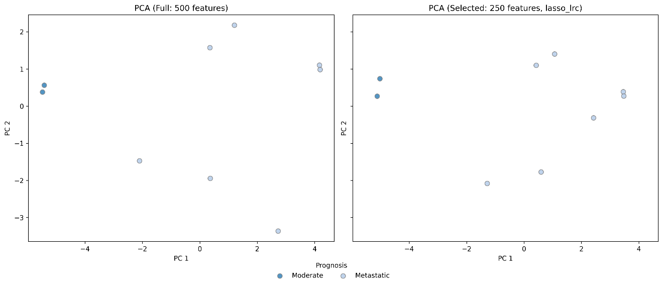
Figure 2. Example of PCA visualization illustrating the effect of CpG feature selection. In this case, Lasso logistic regression was applied to a dataset containing two prognostic categories, Moderate and Metastatic . The left plot shows the PCA projection using all 500 CpG features, while the right plot displays the projection after retaining the top 250 ranked features. Each point represents a sample, colored according to its prognostic category. After feature selection, the two groups become more distinguishable, demonstrating the enhanced separability achieved through the ranking process.

Differential methylation point (DMP) analysis is performed using the limma package (Adams et al., 2023) , which applies linear modeling to identify CpG sites exhibiting significant methylation differences between two user-defined biological conditions. The user specifies which two categories of the target or output variable to compare, such as disease states, treatment groups, or prognostic outcomes. The analysis uses a matrix of methylation β-values, from which a design matrix is constructed to represent the selected conditions. For each CpG site, a linear model is fitted to estimate the difference in average methylation (Δβ or deltaBeta ) between the two groups. A contrast matrix isolates the specific comparison of interest, and empirical Bayes moderation is applied to improve the precision of variance estimates and increase the reliability of differential detection, particularly when the number of samples is limited. The resulting statistics include both Δβ values and p -values for every CpG site, reflecting the magnitude and significance of methylation changes, respectively. Both thresholds are defined by the user, allowing customization of the analysis according to the desired stringency level. CpG sites with positive Δβ values exceeding the chosen threshold are classified as hypermethylated in the first condition, whereas those with negative Δβ values below the threshold are considered hypomethylated. By enabling user control over the compared conditions and statistical cutoffs, this approach provides flexibility and adaptability across diverse methylation studies.

Following DMP analysis, the results are visualized using a volcano plot to provide an overview of methylation differences between the selected conditions. Each point on the plot represents a CpG site, positioned according to its deltaBeta value on the x-axis and the negative logarithm of its p -value on the y-axis. This two-dimensional representation allows simultaneous evaluation of both the magnitude and statistical significance of methylation changes. CpG sites that exceed the user-defined Δβ and p -value thresholds are highlighted, with those exhibiting positive Δβ values classified as hypermethylated and those with negative Δβ values as hypomethylated. Dashed reference lines mark the applied thresholds, clearly separating significant from non-significant CpG sites. The plot also labels the most prominent differentially methylated positions, allowing rapid identification of candidate loci for downstream biological interpretation. Through this visualization, users can intuitively assess how the chosen thresholds influence the overall distribution of methylation changes and identify CpG sites that contribute most strongly to the observed differences between the compared biological conditions. This visualization is implemented through the ggplot2 and ggrepel R packages.

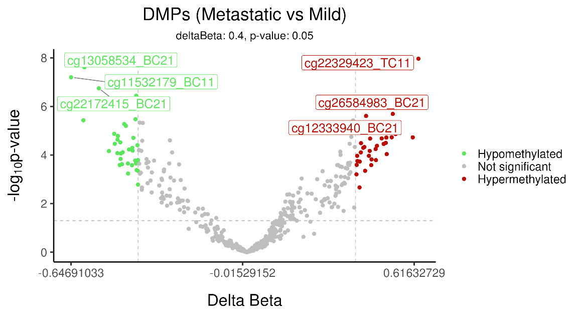
Figure 3. Example of a volcano plot generated after differential methylation point (DMP) analysis using the limma package. In this example, the comparison is performed between the Metastatic and Mild categories, with user-defined thresholds of Δβ = 0.4 and p -value = 0.05. Each point represents a CpG site, plotted by its Δβ value on the x-axis and the negative logarithm of its p -value on the y-axis. Green points indicate hypomethylated sites, red points correspond to hypermethylated sites, and grey points represent CpG sites that do not meet the specified significance criteria. The labeled CpG sites denote the most statistically significant differentially methylated positions identified in this comparison.

After either DMP analysis or AI-based feature ranking, gene mapping is conducted to associate the selected CpG sites with their corresponding gene symbols. The process relies on Illumina methylation array annotations (450K, EPIC, or EPICv2) to accurately match each CpG identifier to its annotated gene. Based on the array type used, the CpG sites retained from the previous analytical step are cross-referenced with the appropriate annotation dataset, and the corresponding gene symbols are extracted. This step ensures that the selected CpG sites are linked to biologically meaningful entities, allowing the transition from probe-level findings to gene-level interpretation. The resulting output provides a comprehensive table containing each CpG site alongside its associated gene symbol, serving as the foundation for subsequent biological or functional analyses.

Following gene mapping, enrichment analysis is performed using the Enrichr API to identify biological pathways and functional categories associated with the mapped genes. The implementation, developed in JavaScript, interfaces directly with Enrichr’s cloud-based API to automate data upload, processing, and retrieval of enrichment results. Gene lists derived from the mapping step are read from CSV files, parsed through the PapaParse library, and uploaded to Enrichr using HTTP POST requests via the /addList endpoint. Once processed, enrichment results are fetched in tab-delimited format through the /export endpoint, enabling the extraction of key metrics such as p-values , combined scores , and gene overlap counts . The tool dynamically retrieves available pathway libraries (e.g., Reactome, KEGG, WikiPathways, BioPlanet) through the Enrichr /datasetStatistics endpoint and allows users to select the preferred database for enrichment computation. The output is rendered interactively, displaying the top-ranked pathways based on statistical significance or combined score. This approach provides a reproducible and automated workflow that bridges methylation-based CpG selection with downstream functional interpretation, helping to identify biologically relevant pathways enriched in the selected gene sets .

Garson, G. D. (1991). Interpreting neural network connection weights. Artificial Intelligence Expert, 6(4), 46–51.

Olden, J. D., Jackson, D. A., & Joy, M. K. (2004). An accurate comparison of methods for quantifying variable importance in artificial neural networks using simulated data. Ecological Modelling, 178(3–4), 389–397.

Azman, N. S., Samah, A. A., Lin, J. T., Majid, H. A., Shah, Z. A., Wen, N. H., & Howe, C. W. (2023). Support vector machine–recursive feature elimination for feature selection on multi-omics lung cancer data. Progress in Microbes & Molecular Biology, 6(1).

Huang, Z., & Chen, D. (2021). A breast cancer diagnosis method based on VIM feature selection and hierarchical clustering random forest algorithm. IEEE Access, 10, 3284–3293.

Khan, M. H., Bhadra, A., & Howlader, T. (2019). Stability selection for lasso, ridge and elastic net implemented with AFT models. Statistical Applications in Genetics and Molecular Biology, 18(5).

Zhang, J., Ma, X., Zhang, J., Sun, D., Zhou, X., Mi, C., & Wen, H. (2023). Insights into geospatial heterogeneity of landslide susceptibility based on the SHAP-XGBoost model. Journal of Environmental Management, 332, 117357.

Friedman, J. H., Hastie, T., & Tibshirani, R. (2010). Regularization paths for generalized linear models via coordinate descent. Journal of Statistical Software, 33, 1–22.

Greenacre, M., Groenen, P. J., Hastie, T., d’Enza, A. I., Markos, A., & Tuzhilina, E. (2022). Principal component analysis. Nature Reviews Methods Primers, 2(1), 100.

Adams, C., Nair, N., Plant, D., Verstappen, S. M., Quach, H. L., Quach, D. L., Carvidi, A., Nititham, J., Nakamura, M., Graf, J., & Barton, A. (2023). Identification of cell-specific differential DNA methylation associated with methotrexate treatment response in rheumatoid arthritis. Arthritis & Rheumatology, 75(7), 1088–1097.